GEEDEF is a cloud-based, interactive land cover classification tool built entirely within the Google Earth Engine (GEE) Code Editor using the GEE JavaScript API. It is designed to accelerate supervised land cover mapping workflow with full GUI panel
Repositori di GitHub · Halaman web
Platform: Google Earth Engine (JavaScript API) | Data: Sentinel-2A SR Harmonized | Version: V3.1






🆕 What’s New in V3.1
Updated from V3 (original PDF release). The following features were added in the latest version accessible via the updated GEE link.
| # | New Feature | Description |
|---|---|---|
| 1 | 📥 Import Training Samples from SHP Asset | Fully new sub-panel in Step 4 — load existing training data from a GEE FeatureCollection asset (uploaded SHP), auto-read attribute columns, extract unique classes, map class codes and names, and merge with manually digitized samples |
| 2 | 📖 Read Columns | Dedicated button to read and populate attribute column dropdowns from the selected SHP asset — eliminates manual column name entry |
| 3 | 🔍 Extract Unique Classes | Scans the selected SHP asset for all unique numeric class codes and renders an editable row per class (name + color) before import |
| 4 | 🔄 Dual Asset Refresh | Separate asset refresh inputs for both the ROI boundary and the training sample SHP — previously only one input field existed |
| 5 | ⚠️ Accuracy Penalty Flag | If only manual samples are used (no field-validated asset imported), the tool applies a −5% correction to OA and Kappa and displays a warning note — makes the reliability of the assessment transparent |
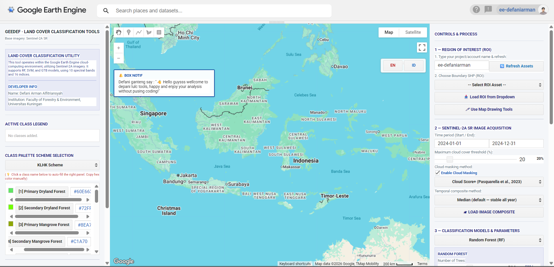
| 6 | 🌐 Bilingual UI (EN / ID) | Full interface toggle between English and Bahasa Indonesia via EN / ID buttons on the map — all labels, buttons, placeholders, and status messages switch dynamically |
| 7 | 📋 Hex Color Copy Box | Each class in the palette panel now renders an editable hex code textbox next to the class button — allows direct copy without needing to memorize or retype the color code |
Overview
GEEDEF is a cloud-based, interactive land cover classification tool built entirely within the Google Earth Engine (GEE) Code Editor using the GEE JavaScript API. It is designed to accelerate supervised land cover mapping workflows at regional and local scales using Sentinel-2A Surface Reflectance (SR) Harmonized imagery.
The tool integrates three scientifically established machine learning classifiers — Random Forest (RF), Gradient Tree Boost (GTB), and Support Vector Machine (SVM) — operating over a 26-variable feature space composed of 10 native spectral bands and 16 derived spectral indices. The entire workflow, from image compositing and sample digitization to accuracy assessment and GeoTIFF export, is executed server-side on Google’s distributed computing infrastructure.
Developed by: Defani Arman Alfitriansyah
Institution: Faculty of Forestry and Environmental Science, Universitas Kuningan
Year: 2025
Table of Contents
Prerequisites
| Requirement | Details |
|---|---|
| GEE Account | Active account at earthengine |
| Internet Connection | Stable connection required for server-side computation |
| ROI Boundary | As a GEE FeatureCollection asset, or drawn manually on the map |
| Domain Knowledge | Basic understanding of land cover concepts and satellite image interpretation |
Interface Layout
GEEDEF uses a three-panel side-by-side layout:
Six-Step Workflow
All six steps must be executed sequentially. Skipping any step will trigger a warning in the status panel.
Step 1 — Define Region of Interest (ROI)
The ROI defines the spatial extent for image collection filtering, classifier training, and area calculation. Two methods are available:
Method A — Load from GEE Asset
Enter your GEE account or project name in the text field (e.g.,
ee-defaniarman).Click 🔄 Refresh Assets to populate the dropdown with available
FeatureCollectionassets.Select the boundary SHP from the dropdown.
Click 📥 Load ROI from Dropdown.
The map centers on the loaded ROI and displays the boundary as a blue outline.
Method B — Manual Drawing
Activate the Drawing Tools from the top-left map toolbar (pencil icon).
Draw a polygon defining your study area boundary.
Click 🖊 Use Map Drawing Tools.
Recommendation: For district-scale or larger study areas, Method A is preferred to ensure administrative boundaries match official data.
Step 2 — Sentinel-2A Composite Acquisition
Builds a cloud-free image composite from COPERNICUS/S2_SR_HARMONIZED according to user-defined parameters.
Acquisition Parameters
| Parameter | Description | Default |
|---|---|---|
| Date Range | Start and end date in YYYY-MM-DD format | 2024-01-01 to 2024-12-31 |
| Cloud Max (%) | Maximum CLOUDY_PIXEL_PERCENTAGE per scene | 20% |
| Cloud Masking | Enable/disable pixel-level cloud masking | Enabled |
| Composite Method | Temporal aggregation strategy | Median |
Cloud Masking Methods
| Method | Description | Recommendation |
|---|---|---|
| Cloud Score+ | Uses cs_cdf layer; masks pixels with cs_cdf < 0.60 | ✅ Recommended — highest accuracy (Pasquarella et al., 2023) |
| SCL (ESA) | Removes SCL classes: cloud shadow (3), unclassified (7), medium cloud (8), high cloud (9), thin cirrus (10), snow/ice (11) | Suitable for most tropical regions |
| QA60 (Bitmask) | Uses bit 10 (opaque cloud) and bit 11 (cirrus cloud) | Simplest but least precise |
Temporal Composite Methods
| Method | Description | Best Use |
|---|---|---|
| Median (Default) | Pixel-wise median across all scenes in date range | Annual mapping; stable and representative |
| Median Dry Season | Selects lowest NDVI quartile (25% driest scenes) | Spectral contrast between open land and vegetation |
| Median Wet Season | Selects highest NDVI quartile (25% greenest scenes) | Maximizing vegetation response |
Step 3 — Classification Algorithm & Parameters
Random Forest (RF)
| Parameter | Range | Default | Description |
|---|---|---|---|
numTrees | 50–1000 | 500 | Number of decision trees |
minLeafPopulation | 1–20 | 1 | Minimum samples per terminal leaf |
bagFraction | 0.3–1.0 | 0.5 | Proportion of samples per tree |
Gradient Tree Boost (GTB)
| Parameter | Range | Default | Description |
|---|---|---|---|
numTrees | 50–500 | 200 | Number of boosting iterations |
shrinkage | 0.01–0.30 | 0.05 | Learning rate |
samplingRate | 0.30–1.0 | 0.7 | Proportion of samples per iteration |
maxNodes | 2–10 | 5 | Maximum depth per tree |
loss | — | LeastAbsoluteDeviation | Loss function |
Support Vector Machine (SVM)
| Parameter | Range | Default | Description |
|---|---|---|---|
kernel | RBF / LINEAR / POLY / SIGMOID | RBF | Kernel function |
cost (C) | 0.1–100 | 10 | Regularization parameter |
gamma | 0.001–2.0 | 0.5 | Influence range (RBF, POLY, SIGMOID) |
degree | 1–10 | 3 | Polynomial degree (POLY only) |
coef0 | 0.0–5.0 | 0.0 | Independent coefficient (POLY, SIGMOID) |
Training / Testing Split
Default 70/30. Use 80/20 for datasets with fewer than 200 samples per class. Minimum 20–30 polygons per class required for statistically valid accuracy evaluation.
Step 4 — Add Classes & Digitize Training Samples
Option A — Import from SHP Asset (New in V3.1)
Enter your GEE account/project name and click 🔄 Refresh to load available SHP assets.
Select the training sample asset from the dropdown.
Click 📖 Read Columns to populate attribute column dropdowns.
Select the class code column and the class name/label column.
Click 🔍 Extract Unique Classes — an editable row appears for each class (name + color).
Edit names and colors as needed, then click 📥 Save & Import Mapped Samples.
Imported samples are merged with any manually digitized samples before training.
Option B — Manual Class Entry
Type a class name, or click a class from the Left Panel palette for auto-fill.
Enter the hexadecimal color code (e.g.,
#006400).Click + ADD CLASS — codes are assigned automatically and increment sequentially.
Digitizing Samples
Select the active class from the dropdown.
Activate Drawing Tools (top-left of map); choose point or polygon.
Draw sample areas on the map for the selected class. Repeat for all classes.
Best practice: Distribute samples spatially. Use multiple small polygons per class to capture within-class spectral variability. Avoid transitional or ambiguous zones.
Step 5 — Run Classification
Click 🚀 RUN CLASSIFICATION. The tool executes server-side:
Extracts spectral values (26 variables) from all samples via
sampleRegionsRandomly splits samples into training / validation sets using
randomColumnTrains the classifier on the training set
Classifies all pixels within the ROI
Computes error matrix → derives OA and Kappa from the validation set
Calculates per-class area via
ee.Image.pixelArea()in hectares
Accuracy Interpretation
| Metric | Threshold | Note |
|---|---|---|
| Overall Accuracy (OA) | > 85% | Generally accepted for regional land cover studies |
| Kappa Coefficient | > 0.80 | “Very Strong” agreement (Landis & Koch, 1977) |
⚠️ If only manual samples are used (no imported field-validated asset), a −5% penalty is applied to OA and Kappa and flagged in the results panel.
Step 6 — Export to Google Drive
Set folder name (default:
GEE_Export) and filename (default:LandCover_DFRF_V3).Select output spatial resolution: 10 m, 20 m, or 30 m.
Click ⬆ EXPORT — GeoTIFF to Drive.
Monitor in the Tasks tab (clock icon, top-right of GEE Code Editor). Click Run.
Output is a single-band integer raster (pixel value = class code), CRS: EPSG:4326. Compatible with QGIS, ArcGIS, and all major GIS software.
Feature Space
After loading the composite, GEEDEF automatically computes 16 spectral indices. Together with 10 native Sentinel-2A bands, the total feature space is 26 predictor variables per pixel.
Native Spectral Bands (10)
| Band | Name | Wavelength | Resolution |
|---|---|---|---|
| B2 | Blue | ~490 nm | 10 m |
| B3 | Green | ~560 nm | 10 m |
| B4 | Red | ~665 nm | 10 m |
| B5 | Red Edge 1 | ~705 nm | 20 m |
| B6 | Red Edge 2 | ~740 nm | 20 m |
| B7 | Red Edge 3 | ~783 nm | 20 m |
| B8 | NIR | ~842 nm | 10 m |
| B8A | NIR Narrow | ~865 nm | 20 m |
| B11 | SWIR 1 | ~1610 nm | 20 m |
| B12 | SWIR 2 | ~2190 nm | 20 m |
Derived Spectral Indices (16)
| Index | Full Name | Primary Application |
|---|---|---|
| NDVI | Normalized Difference Vegetation Index | Vegetation density |
| EVI2 | Enhanced Vegetation Index 2 | Canopy structure; reduces atmospheric noise |
| CAI | Cellulose Absorption Index | Bare soil and litter discrimination |
| NDWI | Normalized Difference Water Index | Leaf water content |
| GCVI | Green Chlorophyll Vegetation Index | Chlorophyll estimation |
| SAVI | Soil-Adjusted Vegetation Index | Sparse vegetation over bare soil |
| PRI | Photochemical Reflectance Index | Canopy light use efficiency |
| HALL_COVER | Hall Forest Cover Index | Forest canopy cover estimation |
| IRECI | Inverted Red-Edge Chlorophyll Index | Red-edge based chlorophyll |
| NDRE | Normalized Difference Red Edge | Vegetation health and stress |
| MNDWI | Modified Normalized Difference Water Index | Open water body mapping |
| NDMI | Normalized Difference Moisture Index | Land moisture |
| NDBI | Normalized Difference Built-up Index | Urban and built-up area |
| NBR | Normalized Burn Ratio | Burned area / forest degradation |
| GVS | Green Vegetation Signal | Green vegetation fraction |
| NDFI | Normalized Difference Fraction Index | Forest degradation and fragmentation |
Spectral Index Formulas
Land Cover Palette Schemes
Color swatches below are rendered as inline SVG — visible on GitHub and most Markdown renderers.
🇮🇩 KLHK — Indonesian Ministry of Environment and Forestry
| ID | Class Name | Swatch | Hex |
|---|---|---|---|
| 1 | Hutan Lahan Kering Primer |  | #60E663 |
| 2 | Hutan Lahan Kering Sekunder |  | #72FF00 |
| 3 | Hutan Mangrove Primer |  | #8EA704 |
| 4 | Hutan Mangrove Sekunder |  | #C1A700 |
| 5 | Hutan Rawa Primer | | #60E663 |
| 6 | Hutan Rawa Sekunder | | #72FF00 |
| 7 | Hutan Tanaman |  | #D3E598 |
| 8 | Semak Belukar |  | #EBC0A7 |
| 9 | Semak Belukar Rawa | | #EBC0A7 |
| 10 | Pertanian Lahan Kering |  | #F6FFA7 |
| 11 | Pertanian Lahan Kering Campur |  | #EDF500 |
| 12 | Sawah |  | #A8D6FF |
| 13 | Tambak |  | #7AF4F4 |
| 14 | Permukiman Transmigrasi |  | #728EA7 |
| 15 | Perkebunan |  | #E5D298 |
| 16 | Permukiman |  | #686868 |
| 17 | Bandara / Pelabuhan |  | #D60073 |
| 18 | Lahan Terbuka | | #D60073 |
| 19 | Pertambangan |  | #A70400 |
| 20 | Badan Air |  | #D4FCF7 |
| 21 | Rawa |  | #98E5E5 |
| 22 | Savana / Padang Rumput |  | #D5FF02 |
| 23 | Awan |  | #D1D1D1 |
🌿 MapBiomas Indonesia — Collection 3.0
| ID | Class Name | Swatch | Hex |
|---|---|---|---|
| 3 | Formasi Hutan |  | #1f8d49 |
| 5 | Mangrove |  | #04381d |
| 76 | Hutan Rawa Gambut |  | #2f7360 |
| 13 | Tumbuhan Non-Hutan Lainnya |  | #d89f5c |
| 40 | Sawah |  | #c71585 |
| 35 | Sawit |  | #9065d0 |
| 9 | Kebun Kayu |  | #7a5900 |
| 21 | Pertanian Lainnya |  | #ffefc3 |
| 30 | Lubang Tambang |  | #9c0027 |
| 24 | Permukiman |  | #d4271e |
| 25 | Non-Vegetasi Lainnya |  | #db4d4f |
| 31 | Tambak |  | #091077 |
| 33 | Sungai, Danau, Laut |  | #2532e4 |
🇺🇸 NLCD — National Land Cover Database (USGS)
| ID | Class Name | Swatch | Hex |
|---|---|---|---|
| 11 | Open Water |  | #466b9f |
| 12 | Perennial Ice/Snow |  | #d1def8 |
| 21 | Developed, Open Space |  | #dec5c5 |
| 22 | Developed, Low Intensity |  | #d99282 |
| 23 | Developed, Medium Intensity |  | #eb0000 |
| 24 | Developed, High Intensity |  | #ab0000 |
| 31 | Barren Land |  | #b3ac9f |
| 41 | Deciduous Forest |  | #68ab5f |
| 42 | Evergreen Forest |  | #1c5f2c |
| 43 | Mixed Forest |  | #b5c58f |
| 51 | Dwarf Scrub |  | #af963c |
| 52 | Shrub/Scrub |  | #ccb879 |
| 71 | Grassland/Herbaceous |  | #dfdfc2 |
| 72 | Sedge/Herbaceous |  | #d1d182 |
| 73 | Lichens |  | #a3cc51 |
| 74 | Moss |  | #82ba9e |
| 81 | Pasture/Hay |  | #dcd939 |
| 82 | Cultivated Crops |  | #ab6c28 |
| 90 | Woody Wetlands |  | #b8d9eb |
| 95 | Emergent Herbaceous Wetlands |  | #6c9fb8 |
Tips and Troubleshooting
General Tips
Test with a small ROI first before processing large areas to avoid computation time-outs.
Use Cloud Score+ as the primary masking method for tropical regions like Indonesia, where thin cirrus and coastal aerosols are common.
For mangrove studies, use Median Dry Season composite to maximize spectral contrast between mangrove canopy and aquaculture ponds (tambak).
Distribute samples spatially across the study area. Avoid concentrating all samples in one geographic location.
For SVM with RBF kernel, perform a manual grid search over
Candgammabefore the final classification run.
Common Issues
| Error / Issue | Solution |
|---|---|
"Computation timed out" | Reduce ROI extent; increase scale to 20 or 30 m; shorten the date range |
"Not enough pixels in region" | Use 10 m scale or enlarge the sample polygon area |
| OA very low (< 70%) | Check sample placement; avoid transitional zones; add more samples; merge spectrally similar classes |
| Class missing from output | Ensure all classes have drawn polygons before clicking Run Classification |
| Error loading ROI from asset | Verify full asset path; asset must be FeatureCollection; check sharing/access settings |
| Map layer not appearing | Open Layer Manager (top-right of map); enable all layers; zoom out if ROI is small |
Full Script Repository
https://
Default Configuration (CFG object)
var CFG = {
  startDate:         '2024-01-01',
  endDate:           '2024-12-31',
  cloudMax:          20,
  classProp:         'lc',
  seed:              42,
  scale:             10,
  maxPix:            1e13,
  splitRatio:        0.7,
  // Random Forest
  rf_numTrees:       500,
  rf_minLeaf:        1,
  rf_bagFraction:    0.5,
  // Gradient Tree Boost
  gtb_numTrees:      200,
  gtb_shrinkage:     0.05,
  gtb_samplingRate:  0.7,
  gtb_maxNodes:      5,
  gtb_loss:          'LeastAbsoluteDeviation',
  // Support Vector Machine
  svm_kernel:        'RBF',
  svm_gamma:         0.5,
  svm_cost:          10,
  svm_degree:        3,
  svm_coef:          0.0
};
Cloud Masking Functions
function maskByCSPlus(image) {
  return image.updateMask(image.select('cs_cdf').gte(0.60));
}

function maskBySCL(image) {
  var scl = image.select('SCL');
  return image.updateMask(
    scl.neq(3).and(scl.neq(7)).and(scl.neq(8))
       .and(scl.neq(9)).and(scl.neq(10)).and(scl.neq(11))
  );
}

function maskByQA60(image) {
  var qa = image.select('QA60');
  return image.updateMask(
    qa.bitwiseAnd(1 << 10).eq(0).and(qa.bitwiseAnd(1 << 11).eq(0))
  );
}
Export Configuration
Export.image.toDrive({
  image:          STATE.classifiedImg,
  description:    'LandCover_DFRF_V3',
  folder:         'GEE_Export',
  fileNamePrefix: 'LandCover_DFRF_V3',
  region:         STATE.roi.geometry(),
  scale:          10,           // options: 10, 20, 30
  crs:            'EPSG:4326',
  maxPixels:      1e13,
  fileFormat:     'GeoTIFF'
});
Scientific References
Auriga Nusantara. (2024). Algorithm Theoretical Basis Document (ATBD) MapBiomas Indonesia Koleksi 3 Versi 1. MapBiomas Indonesia.
Breiman, L. (2001). Random forests. Machine Learning, 45(1), 5–32.
Cardille, J. A., Crowley, M. A., Saah, D., & Clinton, N. E. (Eds.). (2024). Cloud-based remote sensing with Google Earth Engine: Fundamentals and applications. Springer International Publishing. Springer International Publishing (2024)
Cortes, C., & Vapnik, V. (1995). Support-vector networks. Machine Learning, 20(3), 273–297.
Friedman, J. H. (2001). Greedy function approximation: A gradient boosting machine. Annals of Statistics, 29(5), 1189–1232.
Gorelick, N., Hancher, M., Dixon, M., Ilyushchenko, S., Thau, D., & Moore, R. (2017). Google Earth Engine: Planetary-scale geospatial analysis for everyone. Remote Sensing of Environment, 202, 18–27. Gorelick et al. (2017)
Kementerian Lingkungan Hidup dan Kehutanan Republik Indonesia. (2024). Keputusan Menteri Lingkungan Hidup dan Kehutanan Nomor 399 Tahun 2024 tentang Standar Penyebarluasan Informasi Geospasial Tematik Lingkup KLHK. KLHK.
Landis, J. R., & Koch, G. G. (1977). The measurement of observer agreement for categorical data. Biometrics, 33(1), 159–174.
Pasquarella, V. J., Brown, C. F., Czerwinski, W., & Rucklidge, W. J. (2023). Comprehensive quality assessment of optical satellite imagery using weakly supervised video learning. In Proceedings of the IEEE/CVF Conference on Computer Vision and Pattern Recognition (pp. 2125–2135). Pasquarella et al. (2023)
U.S. Geological Survey. (2025). Annual National Land Cover Database (NLCD) Collection 1 Science Product User Guide (Version 1.1). USGS.
U.S. Geological Survey. (n.d.). National Land Cover Database (NLCD) class legend and description. USGS.
This tool is released for academic and educational use. All imagery access is subject to Google Earth Engine Terms of Service and Copernicus Sentinel-2 data policies.
- Cloud-Based Remote Sensing with Google Earth Engine: Fundamentals and Applications. (2024). Springer International Publishing. 10.1007/978-3-031-26588-4
- Gorelick, N., Hancher, M., Dixon, M., Ilyushchenko, S., Thau, D., & Moore, R. (2017). Google Earth Engine: Planetary-scale geospatial analysis for everyone. Remote Sensing of Environment, 202, 18–27. 10.1016/j.rse.2017.06.031
- Pasquarella, V. J., Brown, C. F., Czerwinski, W., & Rucklidge, W. J. (2023). Comprehensive quality assessment of optical satellite imagery using weakly supervised video learning. 2023 IEEE/CVF Conference on Computer Vision and Pattern Recognition Workshops (CVPRW), 2125–2135. 10.1109/cvprw59228.2023.00206