This notebook demonstrates the implementation of the Automatic Mangrove Map and Index (AMMI) algorithm using Python-based geospatial tools on Google Earth Engine (GEE).
Based on: Suyarso & Avianto (2022) | Platform: Google Earth Engine + Python




Overview
This notebook demonstrates the implementation of the Automatic Mangrove Map and Index (AMMI) algorithm using Python-based geospatial tools on Google Earth Engine (GEE). The workflow encompasses cloud-masked Sentinel-2 imagery compositing, AMMI index computation, mangrove binary classification, and canopy density visualization — all rendered as publication-quality static maps using cartoee.
The AMMI algorithm was developed specifically for mangrove ecosystems and has been validated in Indonesian coastal settings, including the Aru Islands and the Musi River Delta, South Sumatra (Suyarso, 2022; Suyarso & Avianto, 2022).
Prepared by: Defani Arman Alfitriansyah — Faculty of Forestry, Universitas Kuningan
Table of Contents
Scientific Background
Mangrove forests occupy the intertidal zones of tropical and subtropical coastlines and provide critical ecosystem services, including carbon sequestration, coastal protection, and biodiversity support. Accurate and automated delineation of mangrove extents from satellite imagery remains methodologically challenging due to spectral overlap with other dense vegetation types and the complexity of coastal environments.
The Automatic Mangrove Map and Index (AMMI) is a purpose-built spectral index that exploits the distinct reflectance behavior of mangrove canopies in the Near Infrared (NIR), Shortwave Infrared 1 (SWIR1), and Red bands. Unlike general-purpose indices such as NDVI or EVI, AMMI incorporates a two-component multiplicative structure that simultaneously suppresses open water and non-mangrove terrestrial signals while amplifying the spectral contrast characteristic of mangrove canopies.
Sentinel-2 Multispectral Instrument (MSI) imagery is well-suited for AMMI computation due to its 10–20 m spatial resolution across the relevant spectral bands and its high revisit frequency (~5 days), enabling temporally dense compositing for cloud-free analysis.
AMMI Formula and Thresholds
The AMMI index is computed from surface reflectance values () of three spectral bands:
| Symbol | Band | Sentinel-2 Band | Wavelength |
|---|---|---|---|
| Near Infrared | B8A | ~865 nm | |
| Shortwave Infrared 1 | B11 | ~1610 nm | |
| Red | B4 | ~665 nm |
Component 1 — Land Delineation
This ratio amplifies terrestrial vegetation signals while suppressing spectral contributions from open water and coastal sediment.
Component 2 — Mangrove Classification
The denominator scaling factor (0.65) is empirically calibrated to separate mangrove reflectance from other coastal woody vegetation.
Complete AMMI Formula
Classification Thresholds
| Output Product | Threshold | Description |
|---|---|---|
| Mangrove Binary Map | Presence/absence classification | |
| Mangrove Density Index | Continuous canopy density visualization |
Note: These thresholds were established by Suyarso & Avianto (2022) based on field validation in Indonesian mangrove ecosystems. Site-specific recalibration may be warranted when applying AMMI in geographically distinct regions.
Dependencies
Install the required libraries before running the notebook:
pip install earthengine-api
pip install geemap
pip install cartopy| Library | Version | Purpose |
|---|---|---|
ee (Earth Engine API) | latest | GEE dataset access and computation |
geemap / geemap.cartoee | ≥0.30 | GEE layer visualization; publication-quality static maps |
matplotlib | ≥3.5 | Figure layout and colorbar rendering |
cartopy | ≥0.21 | Map projections, CRS handling, gridline generation |
Data and Region of Interest
| Parameter | Value |
|---|---|
| Satellite | Sentinel-2 SR Harmonized (COPERNICUS/S2_SR_HARMONIZED) |
| Cloud Masking | Cloud Score+ (GOOGLE/CLOUD_SCORE_PLUS/V1/S2_HARMONIZED), threshold: cs_cdf ≥ 0.60 |
| Cloud Cover Filter | CLOUDY_PIXEL_PERCENTAGE < 20% |
| Temporal Range | 2024-01-01 to 2025-12-01 |
| Composite Method | Pixel-wise median |
| Reflectance Scaling | × 0.0001 (DN → surface reflectance) |
| Region of Interest | GEE Asset: projects/ee-defaniarman/assets/areakajian |
The Cloud Score+ mask (cs_cdf ≥ 0.60) provides a robust probabilistic cloud and cloud-shadow screening approach that outperforms the traditional SCL-based masking for coastal environments where thin cirrus and coastal aerosols are common.
Workflow Summary
Sentinel-2 SR Collection
        │
        ▼
Cloud Score+ Masking (cs_cdf ≥ 0.60)
        │
        ▼
Reflectance Scaling (× 0.0001)
        │
        ▼
Median Composite → Clip to ROI
        │
        ├──► Band Selection: B4 (Red), B8A (NIR), B11 (SWIR1)
        │
        ▼
AMMI Index Computation
        │
        ├──► AMMI > 6  → Binary Mangrove Map
        └──► AMMI > 5  → Canopy Density Index
                │
                ▼
        2×2 Cartoee Publication Map
        (False Color | AMMI Raw | Density | Binary)
Code Walkthrough
1. Library Imports and Earth Engine Initialization
import ee
import geemap.cartoee as cartoee
import matplotlib.pyplot as plt
import cartopy.crs as ccrs
import matplotlib.colors as mcolors
import matplotlib.cm as cm
from matplotlib.patches import Patch

# Cartoee compatibility patch
from cartopy.mpl.geoaxes import GeoAxes
from cartopy.mpl.gridliner import LONGITUDE_FORMATTER, LATITUDE_FORMATTER

cartoee.GeoAxes = cartoee.GeoAxesSubplot = GeoAxes
cartoee.ccrs = ccrs
cartoee.LONGITUDE_FORMATTER = LONGITUDE_FORMATTER
cartoee.LATITUDE_FORMATTER = LATITUDE_FORMATTER

# Authenticate and initialize GEE
ee.Authenticate()
ee.Initialize(project='ee-defaniarman')
The compatibility patch for
cartoeeresolves a known API change in recentcartopyversions whereGeoAxesSubplotwas merged intoGeoAxes.
2. Region of Interest and Image Collection
# Load ROI from GEE asset
batas_wilayah = ee.FeatureCollection("projects/ee-defaniarman/assets/areakajian")

# Load Cloud Score Plus
csPlus = ee.ImageCollection('GOOGLE/CLOUD_SCORE_PLUS/V1/S2_HARMONIZED')

# Cloud masking function
def maskS2CSPlus(image):
    qa = image.select('cs_cdf')
    return image.updateMask(qa.gte(0.60))

# Reflectance scaling function
def scale_image(img):
    return img.multiply(0.0001).copyProperties(img, ['system:time_start'])
3. Sentinel-2 Median Composite
s2_base = (ee.ImageCollection('COPERNICUS/S2_SR_HARMONIZED')
    .filterBounds(batas_wilayah)
    .filterDate('2024-01-01', '2025-12-01')
    .filter(ee.Filter.lt('CLOUDY_PIXEL_PERCENTAGE', 20))
)

s2 = (s2_base
    .linkCollection(csPlus, ['cs_cdf'])
    .map(maskS2CSPlus)
    .map(scale_image)
    .median()
    .clip(batas_wilayah)
)
4. AMMI Index Computation
RED   = s2.select('B4')
NIR   = s2.select('B8A')
SWIR1 = s2.select('B11')

AMMI = s2.expression(
    '((NIR - RED) / (RED + SWIR1)) * ((NIR - SWIR1) / (SWIR1 - (0.65 * RED)))',
    {'NIR': NIR, 'RED': RED, 'SWIR1': SWIR1}
).rename('AMMI')

# Binary map (presence/absence)
AMMI_ts = AMMI.gt(6).selfMask().rename('AMMI_binary')

# Density map (continuous)
AMMI_density = AMMI.updateMask(AMMI.gt(5)).rename('AMMI_density')
5. Visualization Parameters
colors_ammi = ['#0000FF', '#00FFFF', '#FFFF00', '#008000']
ammiVis = {'min': 5, 'max': 25, 'palette': colors_ammi}
fcVis   = {'bands': ['B8A', 'B11', 'B4'], 'min': 0, 'max': 0.3}
binVis = {'palette': ['#008000']}| Color | AMMI Value Range | Interpretation |
|---|---|---|
| 🔵 Blue | ~5 | Low-density / sparse |
| 🩵 Cyan | ~10 | Moderate density |
| 🟡 Yellow | ~18 | High density |
| 🟢 Green | ~25 | Very dense canopy |
6. Publication-Quality 2×2 Map
fig, axs = plt.subplots(
    2, 2, figsize=(15, 15),
    subplot_kw={'projection': ccrs.PlateCarree()},
    layout='constrained'
)

# Panel (a): False Color composite (B8A/B11/B4)
cartoee.add_layer(axs[0, 0], s2, region=region, vis_params=fcVis)

# Panel (b): AMMI raw values
cartoee.add_layer(axs[0, 1], AMMI, region=region, vis_params=ammiVis)

# Panel (c): Mangrove density (AMMI > 5)
cartoee.add_layer(axs[1, 0], AMMI_density, region=region, vis_params=ammiVis)

# Panel (d): Binary mangrove map (AMMI > 6)
cartoee.add_layer(axs[1, 1], AMMI_ts, region=region, vis_params=binVis)

plt.show()
Output Maps
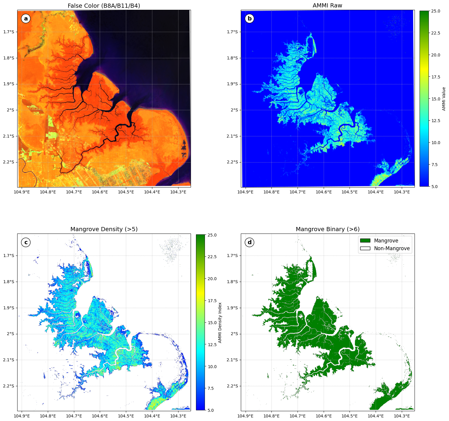
The notebook generates a 2×2 multi-panel figure:
| Panel | Title | Description |
|---|---|---|
| (a) | False Color (B8A/B11/B4) | Standard false-color composite to visually identify mangrove canopy |
| (b) | AMMI Raw | Continuous AMMI values across the full index range |
| (c) | Mangrove Density (>5) | AMMI-derived canopy density index, masked below threshold |
| (d) | Mangrove Binary (>6) | Binary presence/absence classification |
Gridlines are rendered at 0.1° intervals in WGS84 / PlateCarree projection. Colorbars are attached to panels (b) and (c); a categorical legend (Mangrove / Non-Mangrove) is placed on panel (d).
Limitations and Considerations
Threshold generalizability: The AMMI thresholds (
> 5and> 6) were optimized for Indonesian mangrove ecosystems. Application to other biogeographic regions may require field-validated recalibration.Band selection: This implementation uses B8A (red edge NIR, ~865 nm) rather than B8 (~842 nm) for the NIR component. B8A has a narrower bandwidth and is generally preferred for vegetation index computation due to reduced atmospheric noise, though users should verify consistency with the original AMMI formulation.
Temporal compositing: A two-year median composite (2024–2025) minimizes cloud contamination but may smooth phenological variation. Seasonal analyses are recommended for monitoring studies.
No area calculation: This notebook focuses on visualization. For areal extent quantification, apply
ee.Image.reduceRegion()with pixel area weighting (ee.Image.pixelArea()).
References
[1] Gorelick, N., Hancher, M., Dixon, M., Ilyushchenko, S., Thau, D., & Moore, R. (2017). Google Earth Engine: Planetary-scale geospatial analysis for everyone. Remote Sensing of Environment, 202, 18–27. Gorelick et al. (2017)
[2] Hunter, J. D. (2007). Matplotlib: A 2D graphics environment. Computing in Science & Engineering, 9(3), 90–95. Hunter (2007)
[3] Markert, K. (2019). Cartoee: Publication quality maps using Earth Engine. Journal of Open Source Software, 4(33), 1207. Markert (2019)
[4] Met Office. (2015). Cartopy: A cartographic python library with a matplotlib interface. http://
[5] Suyarso. (2022). AMMI Automatic Mangrove Map and Index: An analytical study on satellite imageries at Aru Islands, Maluku, Indonesia. In Emerging Challenges in Environment and Earth Science (Vol. 2, pp. 107–130). BP International. . (2022)
[6] Suyarso, & Avianto, P. (2022). AMMI Automatic Mangrove Map and Index: Novelty for efficiently monitoring mangrove changes with the case study in Musi Delta, South Sumatra, Indonesia. International Journal of Forestry Research, 2022, 1–13. Suyarso & Avianto (2022)
[7] Wu, Q. (2020). Geemap: A Python package for interactive mapping with Google Earth Engine. Journal of Open Source Software, 5(51), 2305. Wu (2020)
Citation
If you use or adapt this notebook in academic work, please cite the primary AMMI methodology:
@article{suyarso2022ammi,
  title   = {AMMI Automatic Mangrove Map and Index: Novelty for efficiently monitoring
             mangrove changes with the case study in Musi Delta, South Sumatra, Indonesia},
  author  = {Suyarso and Avianto, P.},
  journal = {International Journal of Forestry Research},
  volume  = {2022},
  pages   = {1--13},
  year    = {2022},
  doi     = {10.1155/2022/8103242}
}License
This notebook is released for academic and educational use. All data access is subject to Google Earth Engine Terms of Service and Copernicus Sentinel-2 data policies.
Notebook
Notebook dari repositori ini, tampil lengkap dengan sel kode dan hasilnya:
- Gorelick, N., Hancher, M., Dixon, M., Ilyushchenko, S., Thau, D., & Moore, R. (2017). Google Earth Engine: Planetary-scale geospatial analysis for everyone. Remote Sensing of Environment, 202, 18–27. 10.1016/j.rse.2017.06.031
- Hunter, J. D. (2007). Matplotlib: A 2D Graphics Environment. Computing in Science & Engineering, 9(3), 90–95. 10.1109/mcse.2007.55
- Markert, K. (2019). cartoee: Publication quality maps using Earth Engine. Journal of Open Source Software, 4(33), 1207. 10.21105/joss.01207
- . S. (2022). AMMI Automatic Mangrove Map and Index: An Analytical Study on Satellite Imageries at Aru Islands, Maluku, Indonesia. In Emerging Challenges in Environment and Earth Science Vol. 2 (pp. 106–130). Book Publisher International (a part of SCIENCEDOMAIN International). 10.9734/bpi/ecees/v2/3423e
- Suyarso, & Avianto, P. (2022). AMMI Automatic Mangrove Map and Index: Novelty for Efficiently Monitoring Mangrove Changes with the Case Study in Musi Delta, South Sumatra, Indonesia. International Journal of Forestry Research, 2022, 1–14. 10.1155/2022/8103242
- Wu, Q. (2020). geemap: A Python package for interactive mapping with Google Earth Engine. Journal of Open Source Software, 5(51), 2305. 10.21105/joss.02305